Open Source Python GIS
Open Source GIS Libraries
Once you have mastered basic concepts in Python, you are ready to take on working with the GIS libraries. Here is a list of some of the popular open source libraries used in the geospatial community. The list is in no paraticular order. Selection of particular libraries depend on the task that needs to be carried out.
- Geopandas. Great tool. Displays shapefiles with just a few lines of code.
- Rasterio. Simplifies working with raster datasets.
- PyProj.0 Widely used tool for cartographic transformations and geodetic computations
- Cartopy. Cartography library
- Fiona. Reads and write spatial data.
- Shapely. Great for reading and writing spatial data.
- GEOS.. Library for creating Google Earth overlays of tiled maps.
- pyshp. Reads and writes ESRI shapefiles
- GeoDjango. Used for building geospatial web applications
- EarthPy. Simplifies processing of raster and vector data.
- GeoPy. Geocoding library
- PySAL. Used for spatial statistical analysis.
- RSGISLib. Remote Sensing Library
- Geoplot.. Used for plotting maps and several GIS operations.
- PyGeoprocessing. Great for raster processing.
Below, you will find links and code snippets to common tasks in GIS that are made possible using these libraries.
Short Course and Tutorials
- Short Course in manipulating Python Geospatial Libraries
- Intro to Coordinate Reference Systems in Python
- Plotting Coordinates
- Table Joins
- GIS data access and manipulation with Python
- About Vector Data
Code Snippets
Reading and Displaying a Shapefiles Using Geopandas
import matplotlib.pyplot as plt
import geopandas as gpd

file = ".../Michigan_Counties.shp"
df = gpd.read_file(file)

#Display attribute table
print (df)

#Display shapefile
df.plot()

#or
#df.plot(cmap='Set2', figsize=(10, 10));
plt.show() <br>
Plotting a Thematic Map
#import pandas as pd
import geopandas
import matplotlib.pyplot as plt
gdf = geopandas.read_file("/Users/.../Michigan.shp")

#Set up plotting area
f, ax = plt.subplots(1, figsize=(10, 13))

#Display the shapefile
gdf.plot(ax = ax, column= 'MOBILEHOME', cmap='OrRd' , scheme='fisher_jenks', legend=True, edgecolor='black')

ax.set_title("Moble Homes, Michigan", fontdict={'fontsize': '20', 'fontweight' : '3'})

plt.show()

#Save the map
fig.savefig("/Users/.../map_export.png", dpi=300) <br>
Plotting a Shapefile Using PyShp
The geopandas code is preferred over the code below but I include here for the insights it provides into the structure of shapefiles, i.e., parts and points, and how these are accessed and manipulated.
import shapefile as shp
import matplotlib.pyplot as plt

sf = shp.Reader("C:/Users/.../Michigan.shp")

plt.figure(figsize = (10,8))

# loop through each record in the shaperecords collection
for each_rec in sf.shapeRecords():
for i in range(len(each_rec.shape.parts)): #Det the # of parts in each shape to loop through
     #Get the starting and ending values for each part
    i_start = each_rec.shape.parts[i]
    if i==len(each_rec.shape.parts)-1:
        i_end = len(each_rec.shape.points)
    else:
        i_end = each_rec.shape.parts[i+1]

    #Get the X,Y coordinates of the points in each part
    x = [i[0] for i in each_rec.shape.points[i_start:i_end]]
    y = [i[1] for i in each_rec.shape.points[i_start:i_end]]
    plt.plot(x,y, color = "green")

plt.show()
Displaying a Single Band Raster Using GDAL
import numpy as np
import gdal
import matplotlib.pyplot as plt

#Open raster and read number of rows, columns and bands
ds = gdal.Open("/Users/.../TestDEM.tif")

band1 = ds.GetRasterBand(1)

raster_array = band1.ReadAsArray()
plt.imshow(raster_array)
plt.show()
Displaying a Three-band Raster with GDAL
import numpy as np
from osgeo import gdal
import matplotlib.pyplot as plt

aerial = gdal.Open("/Users/.../aerial2.TIF")
bnd1 = aerial.GetRasterBand(1)
bnd2 = aerial.GetRasterBand(2)
bnd3 = aerial.GetRasterBand(3)


#Now turn each band into a ndarray:
img1 = bnd1.ReadAsArray()
img2 = bnd2.ReadAsArray()
img3 = bnd3.ReadAsArray()


#Then stack them to have a 3 band image
img = np.dstack((img1,img2,img3))

plt.imshow(img)
plt.show()
Displaying a Three-band Raster with Rasterio
Rasterio is a popular open source Python library used for viewing and manipulating rasters. Rasterio utilizes the gdal library to display rasters. With rasterio, viewing a raster can be done with just a few lines of code, like the example below.
Rasterio has a show( ) method for displaying rasters. However, the library also uses pyplot’s imshow method to display the data.
import rasterio
from matplotlib import pyplot

src = rasterio.open("C:/Users../N47E010.hgt")
src_array = src.read(1)

fig, ax = pyplot.subplots(1, figsize=(12, 12))
img = ax.imshow(src_array) # Get the plot renderer object.

fig.colorbar(img, ax=ax) #Associate the figure object with plot renderer and axes objects.
ax.set_aspect('auto') #Let the axes object set the length of the colobar.

pyplot.show()
Displaying Satellite Imagery with Rasterio
Calculate Slope and Aspect with Rasterio
First, install the rasterio library To do so, go to the Anaconda prompt and type:
conda install rasterio
Once Rasterio is installed, run the sample script below.
from osgeo import gdal
import numpy as np
import rasterio
import matplotlib.pyplot as plt

def calculate_slope(DEM):
    gdal.DEMProcessing('slope.tif', DEM, 'slope')
    with rasterio.open('slope.tif') as dataset:
        slope = dataset.read(1)
    return slope


def calculate_aspect(DEM):
     gdal.DEMProcessing('aspect.tif', DEM, 'aspect')
     with rasterio.open('aspect.tif') as dataset:
          aspect = dataset.read(1)
     return aspect

slope=calculate_slope("/Users/student/Desktop/TestDEM.tif")
aspect=calculate_aspect("/Users/student/Desktop/TestDEM.tif")

plt.imshow(slope, cmap='copper')
plt.show()
Generate Hillshade Tutorials
- Generate Hillshade
- Generate Hillshade with Earthpy
- Generate Hillshade with Raterrio
- Generate Hillshade with PostGIS
- Generate Hillshade
- Why bother with cpde? Just use QGIS
- Hillshade with GDAL-See Section 2 mostly
Various Raster Processing
Querying Rasters
Find all places with elevation greater than 2500 ft (Method 1)
import gdal
import matplotlib.pyplot as plt

#Open raster and read number of rows, columns, bands
dataset = gdal.Open("C:/Users/.../N47E010.hgt")
band = dataset.GetRasterBand(1)

elevation = band.ReadAsArray(0,0,cols,rows)

a2500 = elevation > 2500

plt.imshow(a2500)
plt.show()
Find all places with elevation greater than 2500 ft (Method 2)
import gdal
import matplotlib.pyplot as plt

#Open raster and read number of rows, columns, bands
dataset = gdal.Open("C:/Users/Hugh/Desktop/N47E010.hgt")
band = dataset.GetRasterBand(1)

cols = dataset.RasterXSize
rows = dataset.RasterYSize

elevation = band.ReadAsArray(0,0,cols,rows)

outData = np.zeros((rows, cols))

for y in range(rows):
     for x in range(cols):
          if elevation[y, x] > 2500:
              outData[y, x] = 1
          else:
              outData[y, x] = 0

plt.imshow(outData)
plt.show()
Perform Neighborhood Analysis
In GIS, many operations are based on neighborhood filters. This illustration below shows notation for a cell and its neightbors. The script that follows shows a basic procedure for accessing and processing neighborhood data based on a 3 x 3 filter.

import gdal
import matplotlib.pyplot as plt
dataset = gdal.Open("N47E010.hgt")
cols = dataset.RasterXSize
rows = dataset.RasterYSize
allBands = dataset.RasterCount
band = dataset.GetRasterBand(1)

elev = band.ReadAsArray(0,0,cols,rows).astype(np.int)

outData = np.zeros((rows, cols), np.int)
for i in range(1,rows-1): # skipping first & last
     for j in range(1,cols-1):
         outData[i,j] = (elev[i-1,j-1] + elev[i-1,j] + elev[i-1,j+1] +  elev[i,j-1] + elev[i,j] + elev[i,j+1] +
                        elev[i+1,j-1] + elev[i+1,j] + elev[i+1,j+1]) / 9.0

print (outData)
plt.imshow(outData)
plt.show()
Kernels for Slope Calculation
Slope calculation in GIS requires the estimation of gradients along two axes. Two methods for calculating gradients are the central differences method and the Horn (1981) method. The former uses the values of two neighboring cells, while the Horn (1981), suitable for rough surfaces, uses the values of six neighboring cells.
Central Differences Method
Gradients along the two axes are calculated as follows:
dz/dx = [ Elev(i, j + 1) - Elev(i, j - 1) ] / 2 cell_size
dz/dy = [ Elev(i - 1, j) - Elev(i + 1, j) ] / 2 cell_size.
In the case of cells at the grid edge, this method can be replaced by the first difference method, in which the central cell itself provides the value for the lateral, missing data.

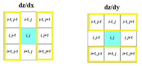
Horn Method
The gradient estimation along an axis derives from the values of six cells in a 3x3 kernel (Fig. 4). The weight applied to each cell depends on its position relative to the central cell. This method is the most suitable for rough surfaces.
dz/dx = [ (Elev(i-1, j + 1) + 2 Elev(i, j + 1) + Elev(i+1, j + 1)) - (Elev(i-1, j - 1) + 2 Elev(i, j - 1) + Elev(i+1, j - 1)] / 8 cell_size
dz/dy = [ (Elev(i - 1, j-1) + 2 Elev(i - 1, j) + Elev(i - 1, j+1)) - (Elev(i + 1, j-1) + 2 Elev(i + 1, j) + Elev(i + 1, j+1)) ] / 8 cell_size
Geoprocessing Rasters
- [Clip and Merge Rasters with GeoRaster](https://pypi.org/project/georasters/